How to Visualize Each Of These Layer Outputs In PyTorch?

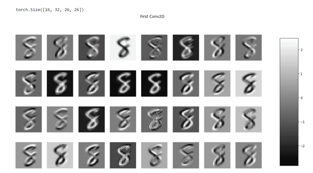
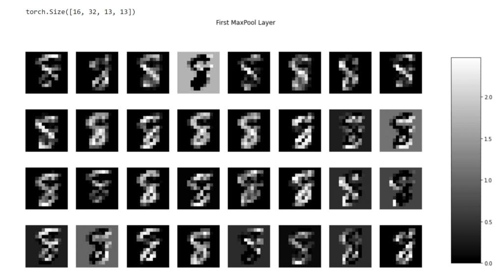
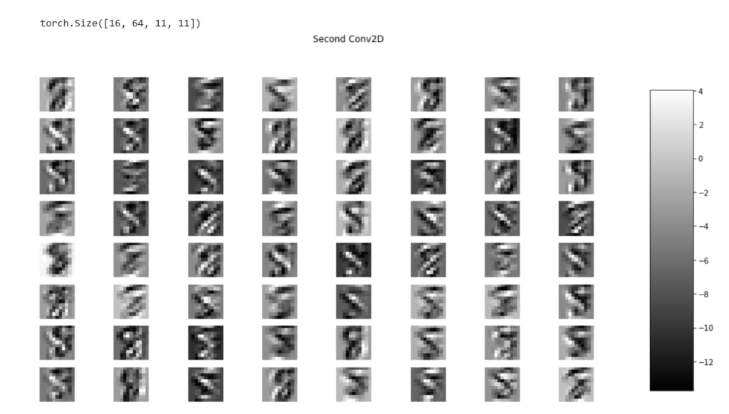
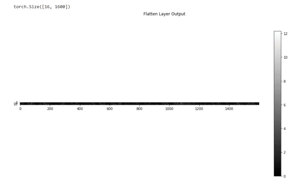
In this article, I build a simple model architecture to train the MNIST ( handwritten 🔠) dataset. After model training is complete then move on to visualize the PyTorch execution graph. The most exciting part of this article is I visualize each of these output layers such as convolution, max pool, linear so on.

Note ⭐ — The main topic in this article is, I visualize each of these layers output. Now it’s time to enough talk, and write some code.

Keep reading 🔥

First Install PyTorch torchviz Libary

Torchviz is a PyTorch library that helps me visualize the execution graph of the model. So my first job is to install this cool✨ library in my notebook.

!pip install torchviz

Import All Necessary Libary Need Achieve This Task

This time I import all the important library needs to complete this task🎯. Once my import is done then move on to the next section for load and transformation.

import torch
import torchvision.datasets as datasets
import torchvision.transforms as transforms
import torch.nn as nn
import numpy as np
import torch
import torch.optim as optim
import matplotlib.pyplot as plt
from torchviz import make_dot
from sklearn.metrics import confusion_matrix
import seaborn as sns


%matplotlib inline

Load MINIST Dataset And Transform Data

device = torch.device('cuda' if torch.cuda.is_available() else 'cpu')

batch_size = 64

# Define the transforms to apply to the data
transform = transforms.Compose([
    transforms.ToTensor(),
    transforms.Normalize((0.1307,), (0.3081,))
])

# Load the MNIST dataset and apply the transforms
train_dataset = datasets.MNIST(root='./data', train=True, download=True, transform=transform)
test_dataset = datasets.MNIST(root='./data', train=False, download=True, transform=transform)

# Create data loaders for the training and test sets
trainloader = torch.utils.data.DataLoader(train_dataset, batch_size=batch_size, shuffle=True)
testloader = torch.utils.data.DataLoader(test_dataset, batch_size=batch_size, shuffle=True)

Let’s understand each of these line codes above 🔥

• device \= torch.device(‘cuda’ if torch.cuda.is_availbale() else ‘cpu’) — I am writing this code because I run my PyTorch code using CPU.

• batch_size — Its simple meaning is how many examples pass through feedforward and backward at a time. For example, suppose your training dataset has 500 examples, and if you set it to batch size 30. This simply means the model doesn’t see the whole dataset one at a time, he only sees 30 examples at a time and repeats this process.

• transform — It is a big topic but I only discuss what I am writing down below. transform.Compose([…]) its technique to transform each of these images sequentially. transform.ToTensor( ) It simply converts the image to a PyTorch tensor. transform.Normalize( ) It simply means to normalize across all the channels with mean and standard deviation.

• datasets.MNIST( ) — I load the popular MNIST dataset that contains 0 to 9 digits.

• root — It’s a directory of the path where you can load this data.

• train — This is set to True mean load train data. If you set it to False mean load test dataset.

• download — I download the dataset internet ( this is set to True )

• transform — It’s a parameter I set of transformations to apply to the dataset. This time I only convert raw data to PyTorch tensor and normalize.

• DataLoader — It’s used to load whole data into batches of PyTorch datasets during training neural networks.

  • dataset — Here’s the actual data you load.

  • batch_size — This specifies how many samples you load per batch.

  • shuffle — If you this parameter set True that means reshuffled at every epoch, default is ( False ).

Display One Image

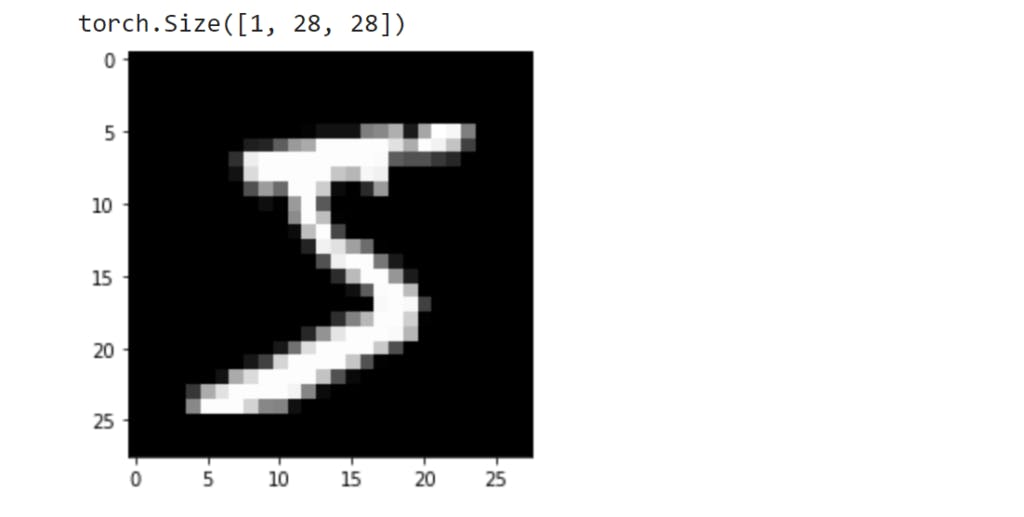
I store trained datasets into DataLoader It’s can be through the iterate datasets. If you get only one image then the syntax looks like this DataLoader.dataset[index number] just like a Python list indexing.

images, label = trainloader.dataset[0]
print(images.shape)
plt.imshow(images.squeeze(),cmap='gray');

Create A Neural Network With PyTorch

class Net(nn.Module):
    def __init__(self, num_classes):
        super(Net, self).__init__()
        self.conv1 = nn.Conv2d(in_channels=1, out_channels=32, kernel_size=3)
        self.relu1 = nn.ReLU()
        self.pool1 = nn.MaxPool2d(kernel_size=2)
        self.conv2 = nn.Conv2d(in_channels=32, out_channels=64, kernel_size=3)
        self.relu2 = nn.ReLU()
        self.pool2 = nn.MaxPool2d(kernel_size=2)
        self.dropout = nn.Dropout(p=0.5)
        self.fc1 = nn.Linear(in_features=1600, out_features=num_classes)
        self.softmax = nn.Softmax(dim=1)

    def forward(self, x):
        x = self.conv1(x)
        x = self.relu1(x)
        x = self.pool1(x)
        x = self.conv2(x)
        x = self.relu2(x)
        x = self.pool2(x)
        x = x.view(x.size(0), -1)
        x = self.dropout(x)
        x = self.fc1(x)
        x = self.softmax(x)
        return x

This architecture under has 2 Convolutional and 2 Relu Activations, 2 max pooling, 1 dropout, 1 linear, and the last 1 softmax activation for predicting a multiclass classification. Every convolution before adding the ReLu activation function.

I do not explain deep this neural network, because this article is not about this topic. But I cover some of them.

Convolutional — in_channels means how many channels have in your image, in my case I am set to 1 means my image is grayscale. out_channels specifies how many filters to apply and the number of channels produce by layer. kernel_size set to 3 simply means 3×3 kernel to compute the output feature map.

Relu Activation — working for activate node when the input value is above zero. If the value is less than zero means is set to zero and greater than zero set itself or simply its model introduces non-linear and increases the expansive power of the model.

MaxPooling Layer — mostly used before the convolution layer because it’s working on downsampling the feature maps. It only gets the highest probability feature map. And this operation reduces the size of the feature and retraining the model’s most important feature.

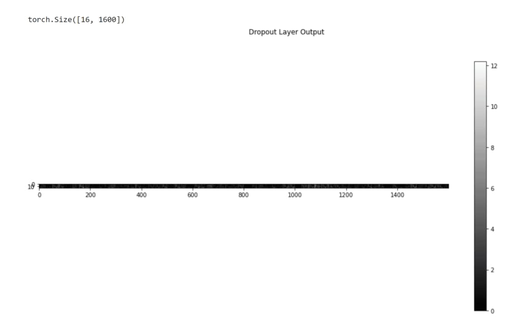
Dropout Layer — It’s mostly used to stop overfitting. and that is randomly dropping some of the neurons every epoch. In my case, I am set to 0.5 which mean is each neuron in the input will have a 50% of probabilities dropped during training time and then pass through the linear layer. Also called it’s maintained by every neuron to learn the same weight means not too high or not too low. For example when you train on a dataset that time some parts of the network learn high weight and others parts don’t much more training. That time turn off the large weight training part and turn on which part does not train on large weights.

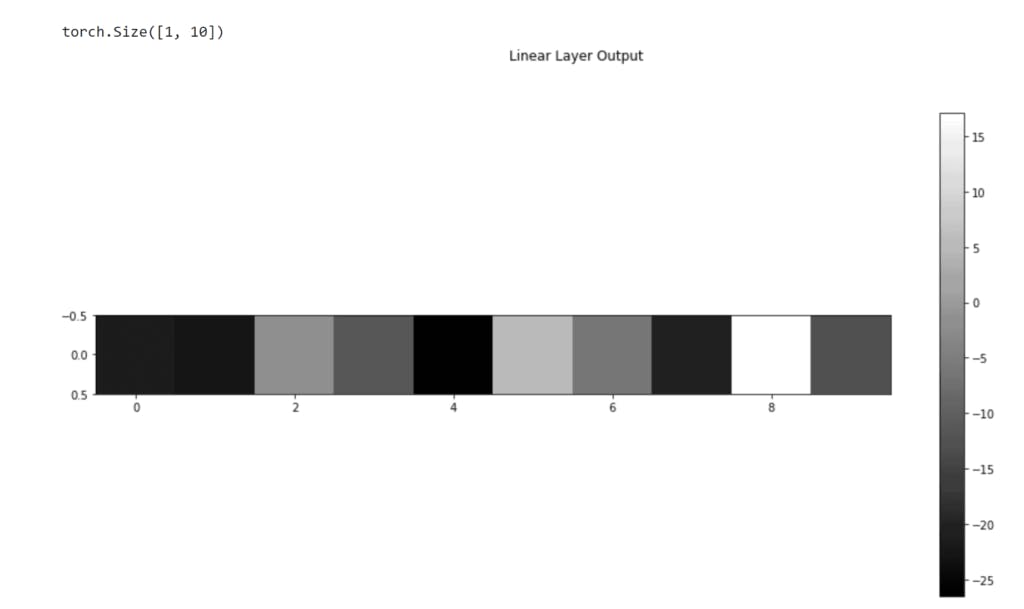
Linear Layer — in_features represents how many input feature you input and out_features represent how many output feature to return. After the linear output feature comes from then passes through the softmax activation function.

Softmax Activation — provides probabilities distribution of the output classes.

Train And Compile Neural Network

If the above neural network class is complete. The next step creates an object of a neural network. Then move on to specify the loss function and optimizer function.

If the above step is complete. Then set how many times to train the model Or simple is the epoch value set. In my case, I am set to 2.

Everything nicely works now loop through and enumerate train data loader. optimizer.zero_grad( ) — Set all gradient values to zero before the gradient computes the next epoch. The main reason for using gradient only looks current mini-batch not looking the previous mini-batch.

Every iterate time passes through data into a model. If successfully set the data, then the model returns the output. This output and actual label input a loss function to calculate loss value.

Then start backpropagation to update the weight and find the best way to decrease to loss value.

net = Net(10)
# Define the loss function
criterion = nn.CrossEntropyLoss()

# Define the optimizer
optimizer = optim.Adam(net.parameters(), lr=0.001)

# Train the model
num_epochs = 2
for epoch in range(num_epochs):
    running_loss = 0.0
    for i, data in enumerate(trainloader, 0):
        inputs, labels = data
        optimizer.zero_grad()
        outputs = net(inputs)
        loss = criterion(outputs, labels)
        loss.backward()
        optimizer.step()
        running_loss += loss.item()
        if i % 100 == 99:
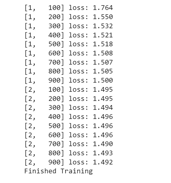
            print('[%d, %5d] loss: %.3f' %
                  (epoch + 1, i + 1, running_loss / 100))
            running_loss = 0.0

print('Finished Training')

Display Model Summary In PyTorch

print(net)

See How To Visualize Execution Graph

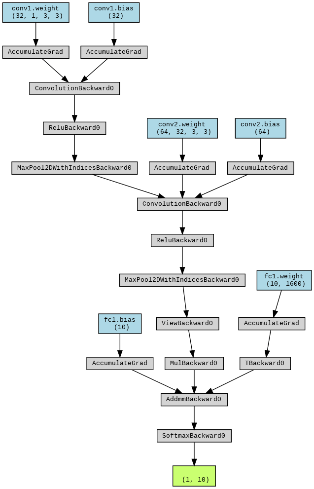
In this section, I use the make_dot( ) function to generate visualized computation graph of my model. This function required the output of the model and the parameter of the model but that is in dictionary format. And then using the render( ) method to specify a file name and format of the image. If works nicely then move on to open this file and see what looks like an actual model execution graph.

images = images.unsqueeze(0)
tag_scores = net(images)

make_dot(tag_scores, params=dict(list(net.named_parameters()))).render("rnn_torchviz", format="png")

Visualize Confusion Matrix

In this section, you see how to create a confusion matrix.

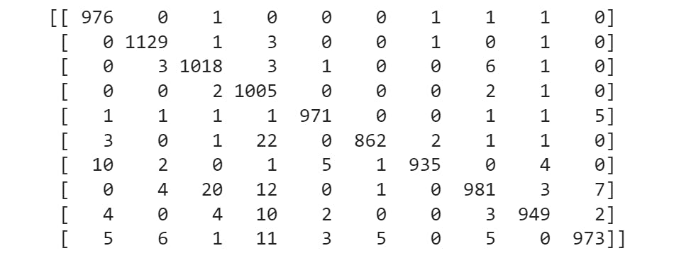
One of the simple ways to build a confusion matrix is just called scikit-learn metrics module that includes the special function name confusion_matrix( ).

# Set the model to evaluation mode
net.eval()

# Create empty lists to store predicted labels and ground truth labels
pred_labels = []
true_labels = []

# Iterate over the test set and predict labels
with torch.no_grad():
    for images, labels in testloader:
        outputs = net(images)
        _, predicted = torch.max(outputs.data, 1)
        pred_labels += predicted.tolist()
        true_labels += labels.tolist()

# Create the confusion matrix
cm = confusion_matrix(true_labels, pred_labels)

# Print the confusion matrix
print(cm)

Now understand the above code 💥

• net.eval() — It’s a mean model set to evaluation mode.

• Create two empty lists for one store’s actual label and another store predicted label

• torch.no_grad() -It’s disabled gradient calculation for validation time. It’s useful to speed up computation and reduces memory usage when a gradient is not needed.

• Loop through the test loader object and get the image and label.

• Now called my model and input the actual image. If the input is set then the model returns probabilities for each of these classes.

• Get the highest probabilities and store them new list name is predicted.

• Convert predicted and actual label torch tensor to Python list.

Predicted and the actual label is ready. And now move on to using the scikit-learn confusion matrix function.

• confusion_matrix()-- It requires two values one is a true label and another is a predicted label.

• I store the confusion matrix value to a new variable and display it.

Visualize Confusion-Matrix With Seaborn

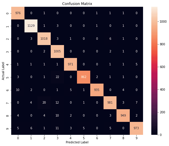
In this section, you learn how to create a color-full way to visualize a confusion matrix.

• First import seaborn library

• Create matplotlib figure

• Create a seaborn heatmap and pass through the confusion matrix. And also set parameters annot=True, and fmt=’d’.

• Set title, xlabel, and ylabel value.

• The final step displays the plot.

plt.figure(figsize=(10,8))
fig = sns.heatmap(cm, annot=True,fmt='d')
plt.title('Confusion Matrix');
plt.xlabel('Predicted Label');
plt.ylabel('Actual Label');
plt.show();

Create Two Visualize Functions

In this section, I create two functions to help visualize layer output. One function visualizes Convulation and MaxPooling layer output. And another function visualize Flatten, Dropout, and Linear layer output.

def conv_max_layer_plot(nrows, ncols, title, image, figsize=(16,8), color='gray'):
  fig, axs = plt.subplots(nrows = nrows, ncols = ncols, figsize=(16, 8))
  fig.suptitle(title)

  for i in range(nrows*ncols):
    image_plot = axs[i//8, i%8].imshow(image[0, :, :, i], cmap=color)
    axs[i//8, i%8].axis('off')
  fig.subplots_adjust(right=0.8)
  cbar_ax = fig.add_axes([0.85, 0.15, 0.05, 0.7])
  fig.colorbar(image_plot, cax=cbar_ax)
  plt.show()


def fdl_layer_plot(image, title, figsize=(16,8)):
  fig, axs = plt.subplots(1 ,figsize = figsize)
  fig.suptitle(title)
  image_plot = axs.imshow(image, cmap='gray')
  fig.colorbar(image_plot)
  axs.axis('on')
  plt.show()

How to Get Single-Layer Output PyTorch

In this section, you see how to get single-layer output. And then rearrange dimensions and convert to a NumPy array.

If the above step is complete then move on to using it above two functions recently created. It displays the output of the layer.

That simple step to follow when you visualize Convulation and MaxPooling layer output.

• The first step is, to call the layer and inputs as an image or it’s not the first layer then inputs as a previous layer output.

• The second step is, to rearrange the output value and convert it to a NumPy array for the compatible matplotlib imshow( ) function. Also, make sure this value stored different variables. Why because this value doesn’t pass to the next layer only used for display.

• The third step is, to call the conv_max_layer_plot( ) function and specify some of the required arguments.

Now follow these steps when you visualize flatten, dropout, and linear layer output.

• The first step is, to call the layer and input as the previous layer output.

• The second step is to convert the PyTorch tensor to a NumPy array. And stored new variables because that value only using for display plots.

The third step is called fdl_layer_plot() and specify some of the required argument.

# Get the output of the first convolutional layer
conv_output = net.conv1(images)
# Rearrange dimensions and convert to numpy array
conv_output_image = conv_output.permute(0, 2, 3, 1).detach().numpy()
print("\n\n",conv_output.shape)
conv_max_layer_plot(nrows=4,ncols=8,title='First Conv2D',image=conv_output_image)

relu_1_output = net.relu1(conv_output)

# MaxPool Layer output visualize
max_pool_output_1 = net.pool1(relu_1_output)
# Rearrange dimensions and convert to numpy array
max_pool_output_image = max_pool_output_1.permute(0, 2, 3, 1).detach().numpy()
print('\n\n',max_pool_output_1.shape)
conv_max_layer_plot(nrows=4,ncols=8,title='First MaxPool Layer',image=max_pool_output_image)

# Get the second convulation output and visualize them
conv_output_2 =  net.conv2(max_pool_output_1)

# Rearrange dimensions and convert to numpy array
conv_output_2_image = conv_output_2.permute(0, 2, 3, 1).detach().numpy()
print('\n\n',conv_output_2.shape)
conv_max_layer_plot(nrows=8,ncols=8,title="Second Conv2D",image=conv_output_2_image)

relu_2_output = net.relu2(conv_output_2)

# MaxPool Layer output visualize
max_pool_output_2 = net.pool2(relu_2_output)
# Rearrange dimensions and convert to numpy array
max_pool_output2_image = max_pool_output_2.permute(0, 2, 3, 1).detach().numpy()
print('\n\n',max_pool_output_2.shape)
conv_max_layer_plot(nrows=8, ncols=8,title='Second MaxPool Layer',image=max_pool_output2_image)

# Flatten Output Visualize
flatten_output = max_pool_output_2.view(max_pool_output_2.size(0), -1)
print('\n\n',flatten_output.shape)
flatten_image= flatten_output.detach().cpu().numpy()
fdl_layer_plot(flatten_image,title='Flatten Layer Output')


dropout_output = net.dropout(flatten_output)
print('\n\n',dropout_output.shape)
dropout_image = dropout_output.detach().cpu().numpy()
fdl_layer_plot(image=dropout_image,title="Dropout Layer Output")

# Linear Layer Output Visualize
linear_1 = net.fc1(dropout_output)
linear_1 = linear_1[0].view(1, -1)
print('\n\n',linear_1.shape)
linear_image = linear_1.detach().cpu().numpy()
fdl_layer_plot(linear_image,title='Linear Layer Output